Programming a simulation of the Earth orbiting the Sun

Please use a newer browser to see the simulation.

"My wonder button is being pushed all the time."

Carl Sagan

This tutorial shows how to program a simulation of the Earth orbiting the Sun with HTML/JavaScript. The complete source code of the simulation can be viewed here. We went through the basics of creating an HTML simulation in the harmonic oscillator tutorial. This tutorial will not be as detailed as the one about the harmonic oscillator. Here we will only discuss the physics and math behind the orbital simulation.

This work is based largely on the concepts from the book by Leonard Susskind and George Hrabovsky “The theoretical minimum: What you need to know to start doing physics”. It is an excellent book that introduces classical mechanics and explains how to write the equations of motion of a system using the Lagrangian and Hamiltonian methods. There are also Susskind’s YouTube video lectures that cover the same material. Please refer to these resources if you want more information on the physics used here.

The coordinate system

We begin by choosing a coordinate system for our simulation. Since the Earth is rotating around the Sun it makes sense to use polar coordinate system shown on Figure 1. The coordinates will be: the angle θ and the distance r between the centers of the Sun and the Earth.

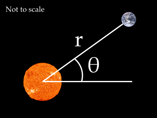
Figure 1: The coordinate system and variables.

The origin of this coordinate system is located at the center of the Sun. This is a simplification, since both the Earth and the Sun rotate around the joint center of mass. However, for the purpose of our simulation we assume that the Sun does not move.

The kinetic and potential energy

The equation for the kinetic energy of the Earth with mass m is

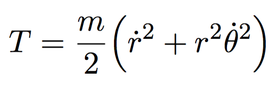(1)

The potential energy, which comes from the gravitational attraction between the Sun of mass M and the Earth, is described by the following equation:

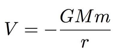(2)

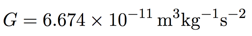
Letter G in Equation 2 is the gravitational constant:

The Lagrangian

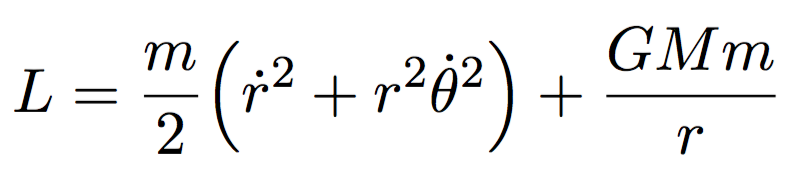
We will find the equations of motions using the Lagrangian, which is the kinetic energy minus the potential energy of the Sun-Earth system:

(3)

The first equation of motion: the distance r

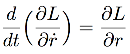
Now we know the Lagrangian and can apply the Euler-Lagrange equation to get two equations of motion. The first one is found using the following formula, involving partial derivatives of the Lagrangian from Equation 3 with respect to distance r and its time derivative:

(4)

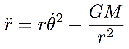
After taking the derivatives we get the first equation of motion:

(5)

We will use Equation 5 in our program and compute the distance r from its second derivative.

The second equation of motion: the angle θ

We use the Euler-Lagrange equation again, but this time we take derivatives of the Lagrangian from Equation 3 with respect to the angle θ and its time derivative:

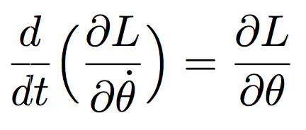(6)

After differentiating and simplifying we get (derivation):

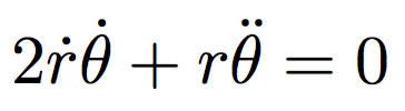(7)

We make the second time derivative of the angle θ the subject of the equation:

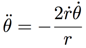(8)

Equation 8 will be used in our program to compute the angle θ from its second derivative.

Solving equations of motions with Euler’s method

We have done the hard part and found Equations 5 and 8, which describe the evolution of the Sun-Earth system over time. In order to animate the Earth we need to solve these equations and find the angle θ and distance r. We will not attempt to solve those differential equations algebraically, but instead use a numerical Euler’s method.

Initial conditions

Before applying the Euler’s method we will first need to set the initial conditions, both for the angle and the distance. We set the initial distance to be equal to the length of the astronomical unit (AU), which is the average distance between the Sun and the Earth. The first time derivative of the distance, or the speed of the Earth, will be zero. Note that this is the speed of the Earth in the direction of the Sun, not the speed in the direction of the orbit.

// Initial condition of the model
var initialConditions = {
  distance: {
    value: 1.496 * Math.pow(10, 11),
    speed: 0.00
  },
  angle: {
    value: Math.PI / 6,
    speed: 1.990986 *  Math.pow(10, -7)
  }
};

Now we need to define the initial conditions of the angle θ. We set an arbitrary value of π/6 radians, since it does not matter at which angle the simulation is started. The value of initial time derivative of the angle θ, or the angular speed, does matter and can be obtained using the following calculation. The Earth makes the full circle in one year, therefore, we can approximate its angular speed by dividing 2π by the number of seconds in the sidereal year.

Storing the current state of the system

The initial conditions describe the system at the start of the simulation. As time changes the Earth will move and the four parameters will change as well. Therefore, in our program we need to store the current state of the system, which is represented by the same four values: position, angle and their time derivatives, or speeds.

var state = {
  distance: {
    value: 0,
    speed: 0
  },
  angle: {
    value: 0,
    speed: 0
  }
};

Computing the acceleration of the distance r

We have set the initial conditions for the distance r and we know how it evolves from Equation 5. Now we can simply write this equation in our program as a function calculateDistanceAcceleration that computes the second time derivative of the distance r given the current state:

function calculateDistanceAcceleration(state) {
  return state.distance.value * Math.pow(state.angle.speed, 2) -
    (constants.gravitationalConstant * state.massOfTheSunKg) / Math.pow(state.distance.value, 2);
}

Computing the acceleration of the angle θ

Similarly, we write the second equation of motion (Equation 8) for the angle as a function calculateAngleAcceleration:

function calculateAngleAcceleration(state) {
  return -2.0 * state.distance.speed * state.angle.speed / state.distance.value;
}

Finding a value from its derivative with Euler’s method

The key feature of the Euler’s method is its ability to compute the value of a physical property from its derivative. For example, the method allows to compute the distance from speed. Similarly, it can give us the speed from the acceleration.

Luckily, this is exactly what we need in our simulation. Equations 5 and 8 give as the accelerations for the distance and the angle respectively. We can then use Euler’s method to find velocities from these accelerations. And by repeating the same trick again, we can find the distance and the angle from their speeds.

To do this, we write a function called newValue. It computes the new value of a physical property by using its derivative and the time increment deltaT:

function newValue(currentValue, deltaT, derivative) {
  return currentValue + deltaT * derivative;
}

In our program, the value deltaT will be a very small time increment, about 90 seconds, which will allow us to approximate the motion of the Earth with reasonable precision.

Finding the distance r

Now we are ready to bring all pieces together and write the code that computes the distance r from its second derivative. First, we use the function calculateDistanceAcceleration to calculate the acceleration r. Then we call newValue to find the speed by using the acceleration. And finally, we use the speed to find the distance r itself:

var distanceAcceleration = calculateDistanceAcceleration(state);

state.distance.speed = newValue(state.distance.speed,
  deltaT, distanceAcceleration);

state.distance.value = newValue(state.distance.value,
  deltaT, state.distance.speed);

Finding the angle θ

We use exactly the same procedure to find the angle θ. First, we find its acceleration with the function calculateAngleAcceleration. Then, we use it to find the angular speed by calling the function newValue. And finally, we compute the angle θ from its angular speed:

var angleAcceleration = calculateAngleAcceleration(state);

state.angle.speed = newValue(state.angle.speed,
  deltaT, angleAcceleration);

state.angle.value = newValue(state.angle.value,
  deltaT, state.angle.speed);

Moving the planet

We have learned how to compute both coordinates r and θ of the Earth. Now all that remains to be done is to run this code repeatedly in a loop and the system will evolve before our eyes. Our program translates the polar coordinates into the actual coordinates of the Earth image on the computer screen and the simulation produces a very natural orbital motion.

I personally find it almost magical that the simulation works at all. Remember that we started with just the Equations 1 and 2 for the kinetic and potential energies of the Sun-Earth system. Then we used those equations to write a Lagrangian equation 3 and find the equations of motions 5 and 8. And finally, we solved those two equations numerically using the Euler’s method. This gave us the precise position of the Earth as the time changes.

For me it is hard to believe that such complex thing as the motion of a planet around its star can be computed so easily from the energy of the system. And yet, it moves.

Credits

1. Editor in chief: Emily Saaen.

2. “The Blue Marble” image: NASA/Apollo 17 crew; taken by either Harrison Schmitt or Ron Evans, source, source.

3. “The Sun photographed at 304 angstroms” image: NASA/SDO (AIA), source, source.

References

• The complete source code of the Earth orbit simulation.

• Susskind, L., & Hrabovsky, G. (2013). The theoretical minimum: What you need to know to start doing physics. New York: Basic Boks.

• Classical mechanics lectures by Leonard Susskind on YouTube.

• Programming a harmonic oscillator.

• Sources of the formulas in LaTex format.