The logistic function
In this article I want to discuss the logistic function that can be used to describe the spread of an infectious disease.
How infection spreads?
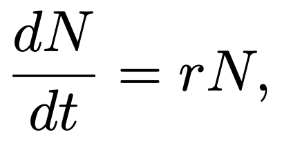
Infectious disease is the one that can spread from human to human. Each sick person can infect healthy people around her. And each of those newly infected people will, in turn, give the virus to even more people. In math language this means that the rate of increase of N (the number of infected people) with time t is proportional to the number of infected people:
 (1)
(1)
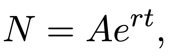
where r is a number that determines how fast infection spreads (i.e. how infectious is the disease). This is a first order linear differential equation, and it has the general solution of the form:
 (2)
(2)
where A is initial number of infected people at time zero, and e is another number equal to about 2.718.
This is a very simple infection model but it can be accurate at the beginning of an epidemic. If we start with just one infected person (A=1) and use rate r=1, then after just five days the number of infected people will be nearly 150 (Fig. 1).
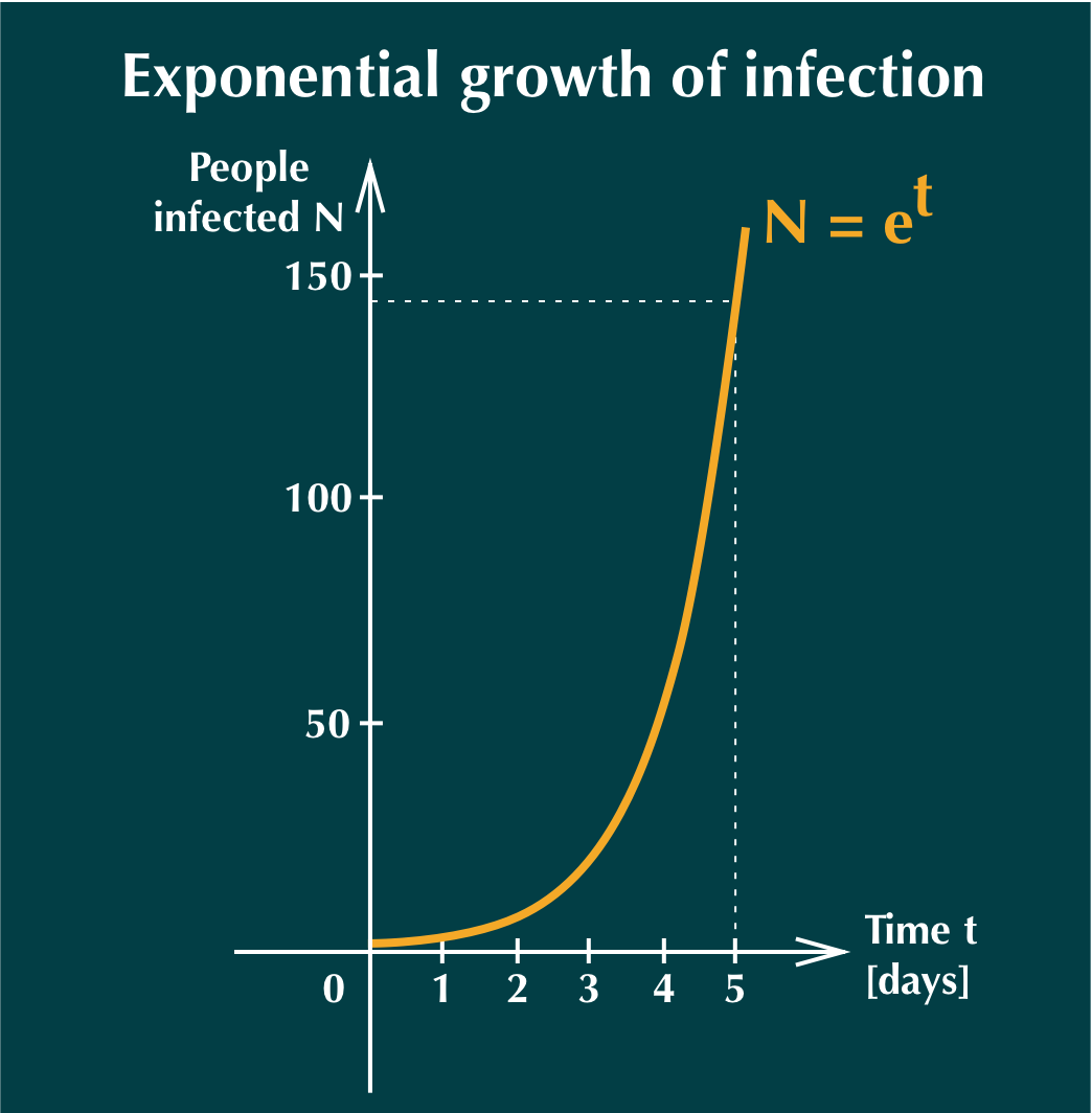
Figure 1: Exponential growth of infection that starts with one infected person.
The virus spreads fast… like a virus. Remarkably, it will take only 23 days until entire population of Earth (nearly 8 billion people) is infected.
What happens when we run out of healthy people? Logistic function happens.
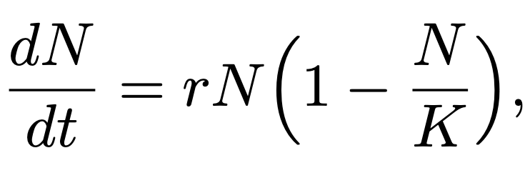
The model shown on Fig. 1 can be very accurate at the start, when most people are healthy. But at some point there will be more ill people around, so there will be more interaction between people who are already infected. As a result, the rate of infection of healthy people will slow down. This can be written in math language as
 (3)
(3)
where K is the total number of people.
At the start of an epidemic, the number of infected people N is small, and therefore Equation 3 gives almost the same result as Equation 1. In other words, at the beginning, Equation 3 describes exponential spread of disease. However, as the number of infected people N gets closer to the total number of people K, the term N/K starts to approach 1, and (1 - N/K) terms approaches zero. Consequently, the rate of change dN/dT also approaches zero. This means that the spread of the disease slows down when many people are ill.
Equation 3 sounds reasonable and it is called logistic growth model. This equation can be solved symbolically to get the general solution:
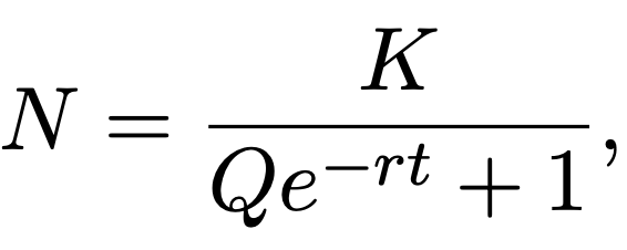 (4)
(4)
where r is the growth rate number, K is total number of people in the population, and Q is a number that relates to the initial number of sick people A as follows:
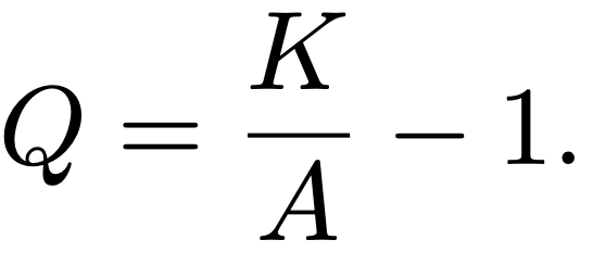 (5)
(5)
Equation 4 is a famous equation and it is called the Logistic Function. Sal Khan has made excellent videos where he shows how to derive it from the logistic growth model (Equation 3).
What does the logistic function look like?
A plot of a logistic function looks like this:
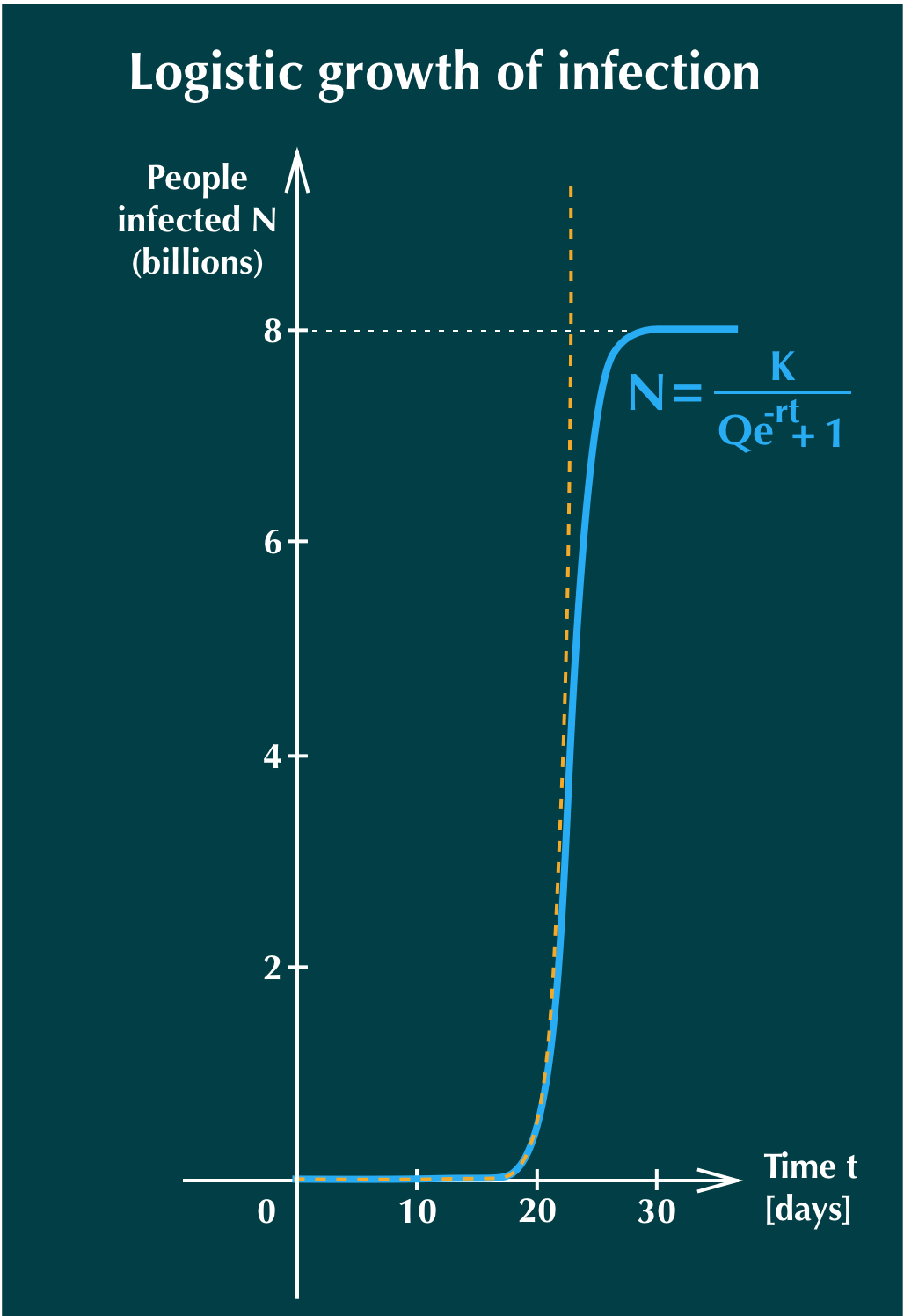
Figure 2: Logistic growth of infection that starts with one infected person (solid blue line). Orange dashed line shows exponential growth, for comparison.
In this plot we used values K=8 billion, r=1 and Q=8 billion - 1. You can try different values on Desmos. We can see that initially, logistic and exponential functions are the same. But after about 20 days the number of infected people starts to grow more slowly for the logistic function, until N levels off at 8 billion people.
Sick! Literally.
Modelling real data
We can use logistic function to model the spread of COVID-19 infection using real data. These data are the number of confirmed cases in different countries at successive days.
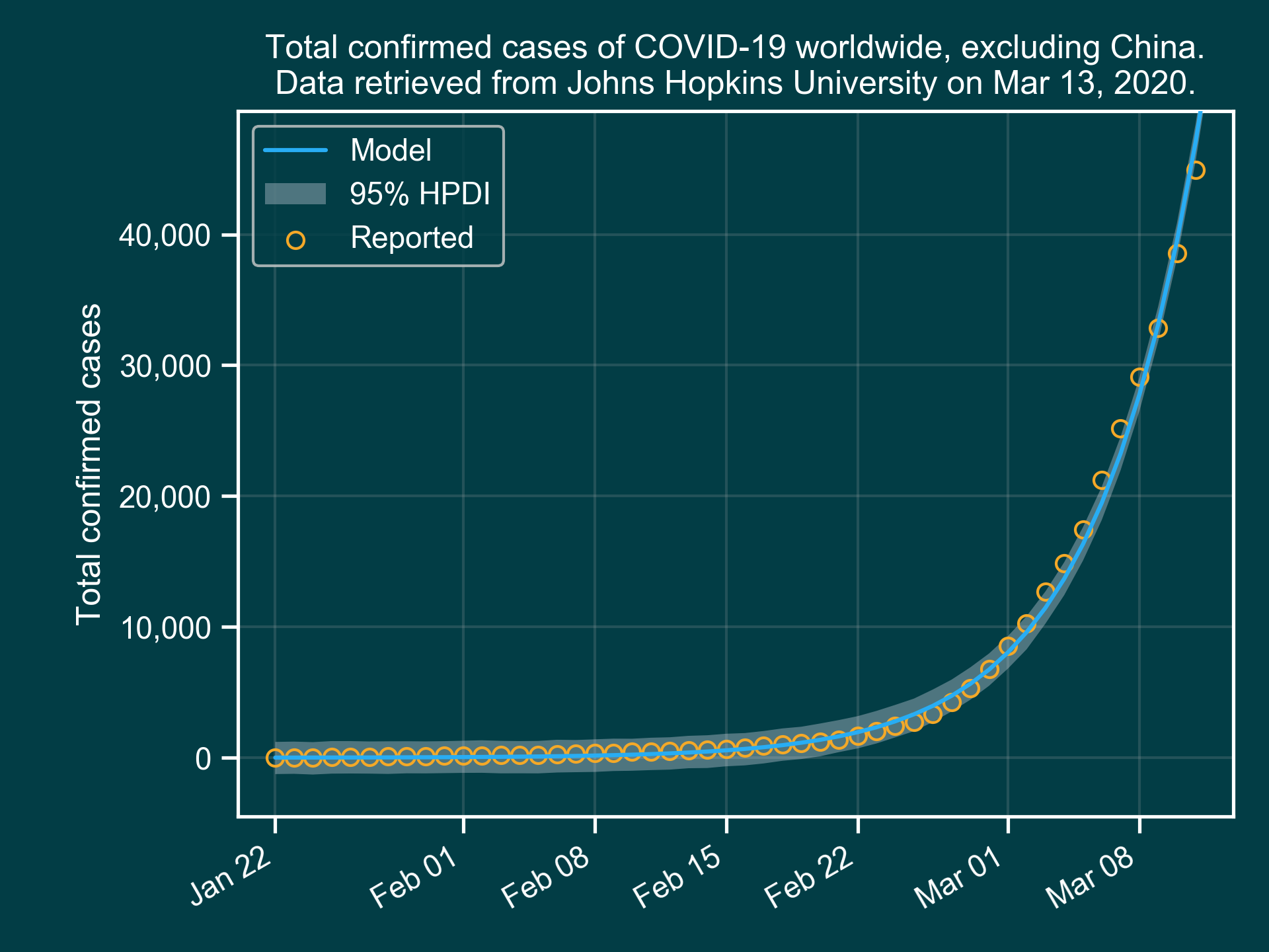
Figure 3: Modeling confirmed cases of COVID-19 worldwide, excluding China.
The orange circles are confirmed cases, and the solid blue line is the model. The bright shaded region around the model line indicates model’s uncertainty.
For this model, we used an arbitrary population size of K=7.8 million. And the initial number of infected people was A=8. The model predicted the growth factor to be around r=0.18. The code for the model is here, and if you want to understand how it works, there is a Statistical Rethinking textbook by Richard McElreath, which is pure gold, in my opinion. :)
Links
-
COVID-19 data from Johns Hopkins University.