Making a JavaScript simulation of two interacting galaxies

Start

What’s this about?

In this post I want to show how to make a simulation of two interacting galaxies that runs in a Web browser, written in HTML, CSS and JavaScript languages. I won’t explain everything, because I would need to write a post ten times longer than it is (and who wants to read that?). Instead, here I just want to briefly show the main ideas that will hopefully make this simulation appear less magical.

Who made this possible?

The idea and the physics code of this simulation are not mine. This work is based on the laboratory manual written by my teacher Daniel Price from Monash University. All I’ve done was port Daniel’s Fortran code to JavaScript and draw in some buttons. Similar simulation was done in 1972 by Alar and Juri Toomre in their Galactic Bridges and Tails paper, an inspiration for Daniel’s simulation.

I also learned how to simulate moving bodies in space from my Monash astronomy teachers Adelle Goodwin, Melanie Hampel, John Lattanzio and Rosemary Mardling (in alphabetical order).

Lastly, most of the 3D code is not mine either, I copy-pasted it from WebGL Funamentals tutorials.

The main idea

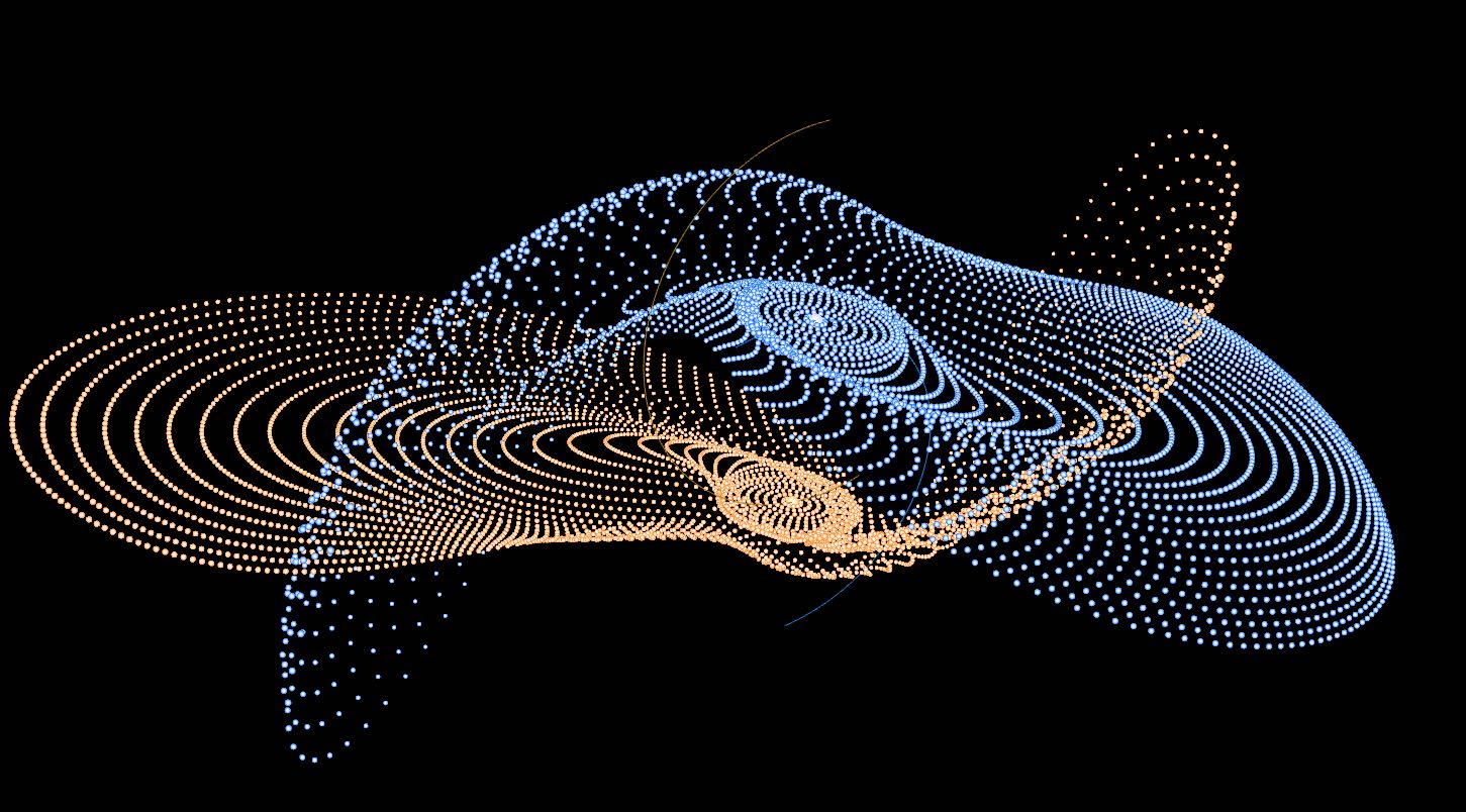
This simulation contains two galaxy cores that move around the common center of mass, located at the origin of the coordinate system (Fig. 1).

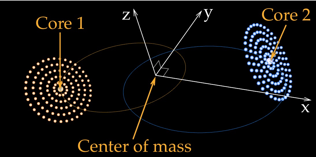
Figure 1: The main idea behind the simulation.

The two cores move in the X-Y plane. If we only consider the cores, then this is just a two-body problem that we coded previously. However, this time we want to add stars that move around each core in circular orbits. The stars form discs that are tilted at adjustable angles with respect to the X-Y plane.

A spherical cow

This model includes a big simplification of reality: the stars in the simulation only feel gravity from the two galactic cores, but not from other stars. This simplification makes the model very unrealistic. In a real galaxy, the mass is not located at the center, but instead contained in the stars and dark matter and distributed throughout the galaxy. For example, our Milky Way contains a supermassive black hole Sagittarius A* in its center, but the black hole is “only” about one millionth (0.000001) of the mass of the galaxy.

But unrealistic simplifications are sometimes useful because they can help us understand something fundamental about nature. For example, it would have been much harder for Galileo and Newton to discover that an unperturbed object moves at constant velocity without ignoring friction and gravity, which are always present in our daily life.

Downloading the code

Enough talking, let’s look at the code, which is located at github.com/evgenyneu/two_galaxies. To download the code, open a Terminal app and run

git clone https://github.com/evgenyneu/two_galaxies.git

This requires Git program to be installed, and it will download the code into two_galaxies directory.

Exploring the code

Open two_galaxies directory in any coding text editor of your choice. I use Atom (Fig. 2), other editors I recommend are Sublime Text and Visual Studio Code.

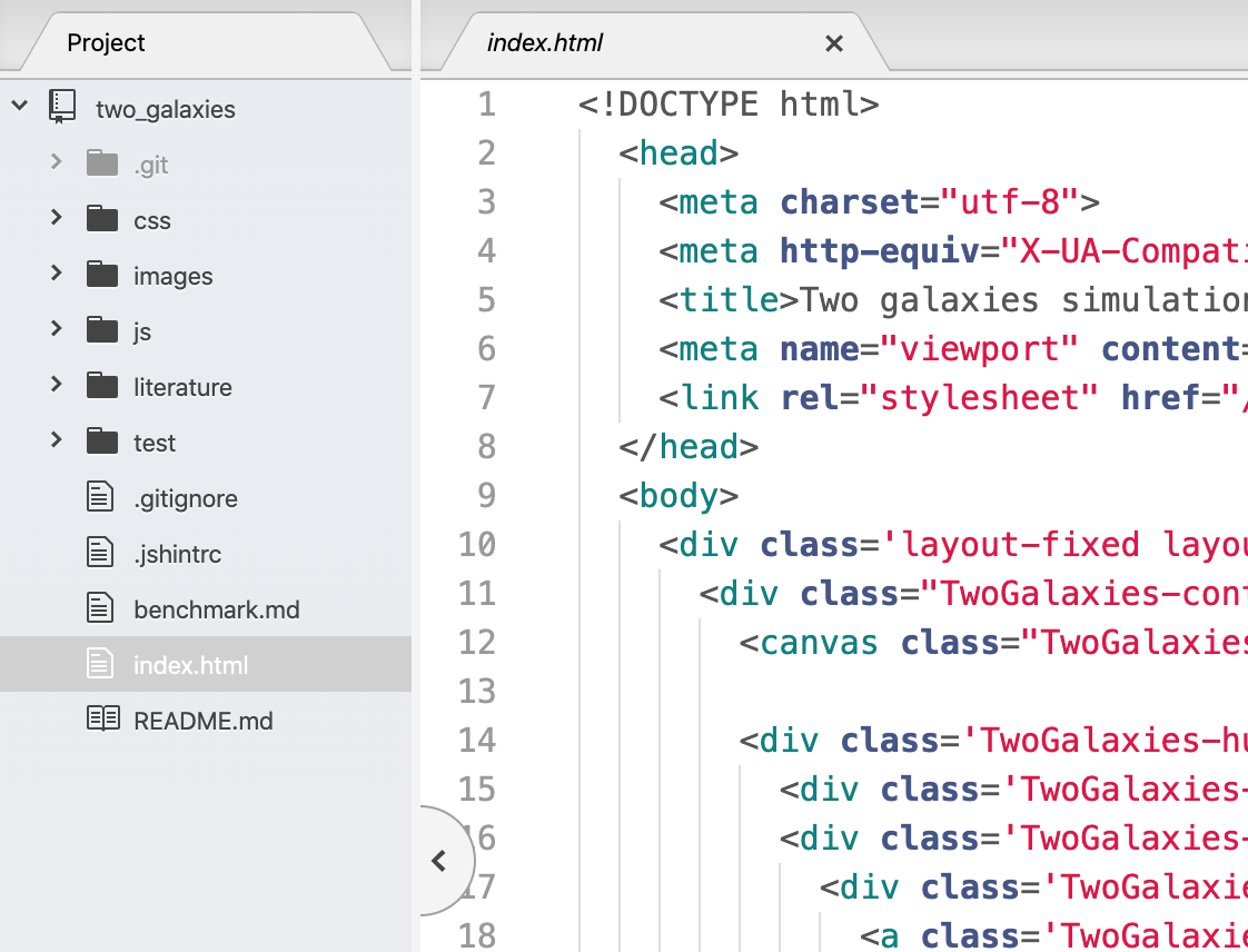
Figure 2: HTML code of the simulation viewed in Atom editor.

The simulation is a web app, and is written in the only three languages any Web browser can understand: HTML, CSS and JavaScript.

HTML code

The HTML code is located in index.html file (Fig. 2). It contains the layout of the web page and its elements, such as the black canvas for drawing stars, buttons and sliders. It also contains code written in GLSL ES language, which stands for OpenGL Shading Language. This code is for showing 3D graphics using the graphics processing unit (GPU). GPU is a computer hardware that is optimised to draw coloured triangles, points and lines on your screen very fast, which makes it possible to animate thousands of stars in real time in this simulation.

CSS code

The CSS code of the simulation is located in css/two_galaxies.css file (Fig. 3). This code is for setting the styles of HTML elements, things like positions, sizes and colors. For example, Fig. 3 shows .TwoGalaxies-button style which is used for all square buttons in the simulation. It sets the size of the buttons to be 45 by 45 pixels.

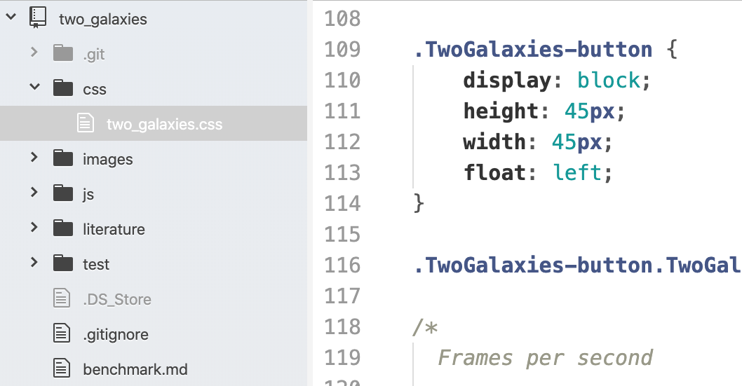
Figure 3: CSS code of the simulation.

JavaScript code

Most of the simulation code is in JavaScript files, located in js directory (Fig. 4). Unlike HTML and CSS, which are languages specific to web development, JavaScript is a general purpose programming language used to encode the logic of a program. For example, Fig. 4 shows a function numberOfStarsInOneRing that calculates the number of stars in a ring of a galaxy. The entry point of the program is located in the main.js file.

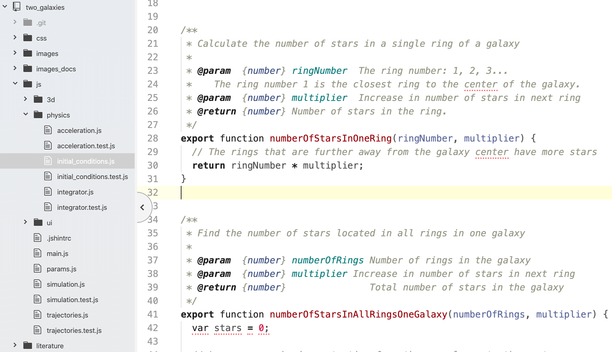
Figure 4: JavaScript code of the simulation.

Run the simulation locally

Next, I want to show how to run the simulation on your computer so you can tinker with the code and see the effects. In order to do this, you need to install a web server, which is a program that runs web sites. There are many web servers available, but the simpler ones come with Python and Node.js.

Option 1: running a web server with Python

First, install Python. Next, in the Terminal, change to the two_galaxies directory where you downloaded the code earlier:

cd two_galaxies

and start the web server:

python -m http.server

You can now open http://0.0.0.0:8000/ URL in your web browser and see the simulation (Fig. 5).

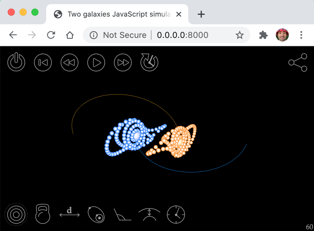
Figure 5: Running the simulation locally using Python web server.

The purpose of using a local web server is that you can make changes to the code, refresh the web browser and see the effects.

Option 2: running a web server with Node.js

Alternatively, instead of Python you can use a web server that comes with Node.js. First, install Node.js. Next, from the Terminal, install the web server:

npm install http-server -g

Finally, from two_galaxies directory, start the web server and navigate to http://127.0.0.1:8080 URL in your web browser to see the simulation:

npx http-server

How the simulation works?

Conceptually, this simulation is very simple. All it is doing is showing moving circles on the screen. The trick is to calculate their positions and then change positions with time. This is done using three steps:

1. First, for each star we calculate three numbers — its x, y, and z coordinates in 3D space — and then use them to draw a coloured circle on screen. These are initial positions of the stars, and that’s where we see them after the web page is first loaded.

2. Next, after a short time interval, we want to calculate new positions using Newton’s second law (we will return to this physics later):

   \[\vec{F} = m \vec{a}. \tag{1}\]

3. Finally, we repeat this 60 times a second (or at a different rate, depending on refresh rate of your monitor), and this gives an impression of a moving collection of stars.

Simple.

Counting the stars

Our first job is to calculate the initial positions of stars. But before that, we need to know the number of stars in each ring of a galaxy (Fig. 6).

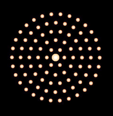
Figure 6: A single galaxy is made of stars placed in circular rings.

This is done with the following function, located in js/physics/initial_conditions.js file:

export function numberOfStarsInOneRing(ringNumber, multiplier) {
  return ringNumber * multiplier;
}

This function returns the number of stars in a given ring of a galaxy. The ring number is passed using input parameter ringNumber, and the increase in the number of stars in each next ring is specified with multiplier parameter. For example, the function will return 6 stars for the first ring when we call numberOfStarsInOneRing(1, 6), 12 for the second ring numberOfStarsInOneRing(2, 6), an so on, adding 6 more stars to the next ring.

Now that you have a local web server running, you can experiment with the code and see the effects. For example, change the return statement from

return ringNumber * multiplier;

to

return 7;

Then refresh the web browser, and you will see funny galaxies shown on Fig. 7.

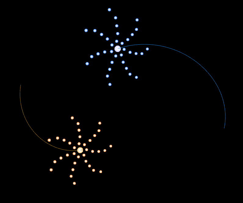
Figure 7: Galaxies with seven stars in each ring.

Next, we need to calculate the total number of stars in one galaxy. This is done by numberOfStarsInAllRingsOneGalaxy function:

export function numberOfStarsInAllRingsOneGalaxy(numberOfRings,
                                                 multiplier) {
  var stars = 0;

  // Loop over each ring, starting from the one closer to the center
  for(let ringNumber = 1; ringNumber <= numberOfRings; ringNumber++) {
    // Calculate the number of stars in one ring and add it to total
    stars += numberOfStarsInOneRing(ringNumber, multiplier);
  }

  return stars;
}

Here, inside the loop, we call function numberOfStarsInOneRing for rings 1, 2, and up to the total number of rings, adding the number of stars in each ring to the galaxy’s total.

Positioning stars in a galaxy

Now that we know the number of stars in one galaxy we can calculate their intial positions and velocities. This is done in galaxyStarsPositionsAndVelocities function located in js/physics/initial_conditions.js file:

export function galaxyStarsPositionsAndVelocities(args) {
  let stars = numberOfStarsInAllRingsOneGalaxy(args.numberOfRings);
  var positions = Array(stars * 3).fill(0);
  var velocities = Array(stars * 3).fill(0);
  ...

It starts with calculating the total number of stars in one galaxy, by calling numberOfStarsInAllRingsOneGalaxy function and saving the result in stars variable. Then it creates two arrays to store positions and velocities of the stars. Since we are dealing with 3D, each coordinate requires three numbers x, y and z. That’s why the size of the arrays is three times larger than the number of stars: Array(stars * 3).

We will need to keep this in mind when accessing positions and velocities form these arrays. For example, positions[0] will be the x-coordinate of the first star and positions[1] will be its y-coordinate. The x-coordinate of the second star is positions[4], and z-coordinate of the seventh star is positions[3*6 + 2], or positions[20], and so on.

Next, we want to set the angle of galaxy inclination (Fig. 8) with respect to the X-Y plane, which is passed to this function as parameter args.galaxyAngleDegree. This angle is chosen by the user in degrees, but we want to convert it to radians, using the fact that 180 degrees is π (3.1415) radians:

var galaxyAngleRadians = args.galaxyAngleDegree * Math.PI / 180;

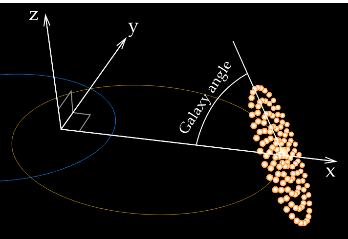
Figure 8: A galaxy inclination angle of 60 degrees. The angle is measured from the X-Y place, where the galaxy cores are moving.

Next, we look at each galaxy ring separately, starting with the first ring using the for loop:

// Loop over the rings of the galaxy
for(let ringNumber = 1; ringNumber <= args.numberOfRings; ringNumber++) {
  // Find distance of stars in current ring from the galaxy center
  let distanceFromCenter = ringNumber * args.ringSeparation;

  // Find number of stars in the ring
  let numberOfStars = numberOfStarsInOneRing(ringNumber,
                                             args.ringMultiplier);

Inside the loop, we calculate the distance of the star (and the ring) from galactic center (Fig. 9), which is equal to the ring number times the separation between rings args.ringSeparation.

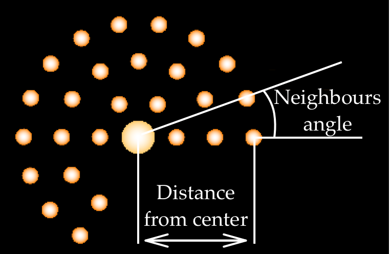
Figure 9: Calculating distance from a star in the third ring to the galactic center and the angle between two neighbours.

We will later need an angle between two neighbouring stars in the same ring, in radians (Fig. 9). To calculate it, we first use numberOfStarsInOneRing function to get the total number of stars in the current ring. Next, we use the fact that the angle of the full ring is 360 degrees, or 2π radians. This means that the angle between two adjacent stars is 2π / numberOfStars:

// Find number of stars in the ring
let numberOfStars = numberOfStarsInOneRing(ringNumber,
                                           args.ringMultiplier);

// Calculate the angle between two neighbouring stars in a ring
// when viewed from the galaxy center
let angleBetweenNeighbours = 2 * Math.PI / numberOfStars;

Calculating initial speeds of the stars

Our goal is to calculate the initial velocity of each star in the galaxy, but first we need to find the speeds of stars. Velocity is a vector, pointing in the direction of movement. The length of a velocity vector is equal to the speed. When the simulation starts, we want our rings to be circular. This means that all stars in the same ring must have equal speeds, otherwise the symmetry of the circle would be broken. Let’s calculate this speed.

Consider a single star. Since we chose to neglect gravity from other stars, the galactic core is the only object that attracts our star (Fig. 10). The core exerts force \(F\) on the star of mass \(m\). This causes the star to accelerate with acceleration \(a\), resulting in a circular orbit instead of a straight line.

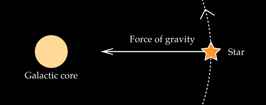
Figure 10: Galactic core exerting gravitational force on an orbiting star.

In math language, this can be expressed with Newton’s second law:

The acceleration \(a\), also called centripetal acceleration, for a body moving in a circle of radius \(r\) with speed \(v\) is given by

Substituting \(a\) into Eq. 2 gives:

Next, we use another of Newton’s discovery - the law of universal gravitation:

which allows us to calculate gravitational force \(F\) between two masses \(m\) and \(M\) that are distance \(r\) apart. Here \(G\) is a number called gravitational constant:

Next, we equate equations 4 and 5:

Mass of the star \(m\) and distance \(r\) cancels:

Finally, we take the square root of both sides and get the expression for the speed of the star we wanted:

Now we return to our galaxyStarsPositionsAndVelocities function, and find this equation in the code:

let starSpeed = Math.sqrt(args.coreMass / distanceFromCenter);

You might have noticed a small difference. Our JavaScript code does not have constant \(G\). Why? Because we made constant \(G\) equal to one.

[reader stares in disbelief]

Let me explain…

Changing units of length, mass and time

You can see that constant \(G\) (Eq. 6) has units of \(\frac{\text{m}^3}{\text{kg} \ \text{s}^2}\). Here \(\text{m}\) (meter) is a unit of length, \(\text{kg}\) (kilogram) is a unit of mass, and \(\text{s}\) (second) is a unit of time. We will now do a trick that I saw astronomers do many times, and which confused me a lot until my teacher John Lattanzio explained it to me.

We want to change the units of length, mass and time in order to make constant \(G\) equal to one in these units.

The point of this is to avoid putting constant \(G\) anywhere in the code. Another reason for this, is to make our mass, length and time numbers small, since stellar masses and distances are very large numbers when expressed in meters and kilograms.

Here is one way of changing the units. We first define the new units

where \(a\), \(b\) and \(c\) are numbers we want to find. Our goal is to make gravitational constant \(G\) equal to one in these units. This is done by taking Eq. 6, replacing the number \(6.67 \times 10^{-11}\) with \(1\) and also replacing \(\text{m}\), \(\text{kg}\) and \(\text{s}\) with new units: \(U_L\), \(U_M\) and \(U_T\):

Next, we substitute new units from Eq. 10:

Equating this with Eq. 6 gives

The units cancel and we get

This equation can not be solved, because it has three unknown variables \(a\), \(b\) and \(c\). Since one of our goals was to make new units small (Eq. 10), we can pick some arbitrary large numbers for \(a\) (length) and \(b\) (mass) and then calculate \(c\) (time) using Eq. 14.

Let’s start with with the length \(U_L\). Stellar distances are often measured with a unit of length called parsec (pc), which is a typical distance between stars:

Galactic distances are even larger, and are often measured in thousands of parsecs, or kiloparsecs (kpc). For example, Earth is eight kiloparsec away from the center of Milky Way. Since we are simulating galaxies, it will make sense to use kiloparsec as our unit of length:

We can now convert kiloparsecs to meters, use Eq. 10 and calculate \(a\):

This gives the new unit of length we were looking for:

Next, we want to choose a suitable value of \(b\) for the unit of mass. We are working with galaxies, so it would be natural to use mass of Milky Way as our mass unit. There are about 300 billion (\(3 \times 10^{11}\)) stars in Milky Way, but we will round it to a 100 billion (\(10^{11}\)). We will assume that the average stellar mass is equal to the mass of the Sun, which is about

Multiplying the Solar mass by the number of stars (\(10^{11}\)) gives the unit of mass we wanted:

Therefore, the number \(b\) is

At last, we can calculate the unit of time by using Eq. 14, substituting numbers \(a\) and \(b\), and finding \(c\):

We have found that in order to make constant \(G\) equal to one in new units (Eq. 11), we need to choose the unit of time to be

This is a very large number, let’s convert it to years, using the fact that there are 3600 seconds in one hour, 24 hours in one day, and 365 days in a typical year:

We have calculated the new unit of time to be 1.5 million years. Let’s see if this number makes sense. Our animation advances by about one unit of time after each animation frame. If refresh rate of the computer screen is 60 frames per second (a typical screen in 2020), then in one second of our time the simulation will advance by 90 million years. This is comparable to the 250 million years, which is the time it takes the Sun to rotate around the center of Milky Way. This means that unit of time \(U_T = 1.5 \times 10^6 \ \text{y}\) is reasonable.

Let’s remind us what we’ve done. Our goal was to get rid of constant \(G\) in code by making it equal to one. We have accomplished this by choosing the following units of length, mass and time, which are also more suitable to galactic scales:

Calculating initial positions of stars in one galaxy

Let’s return to our galaxyStarsPositionsAndVelocities function. Remember, we are inside a loop and want to calculate initial positions of stars for a single ring. We have already calculated the total number of stars numberOfStars in that ring. Now we want to go over all stars in the ring and calculate their positions. We start with another a loop:

// Loop over all the stars in the current ring
for(let starNumber = 0; starNumber < numberOfStars; starNumber++) {
  // Find the angle of the current star relative to the first
  // star in the ring
  let starAngle = starNumber * angleBetweenNeighbours;

Inside the loop we go from the the rightmost star counterclockwise, and we want to calculate the angle to the current star with index starNumber. This angle starAngle is just the star index multiplied by the angle between neighbours, as shown on Fig. 11.

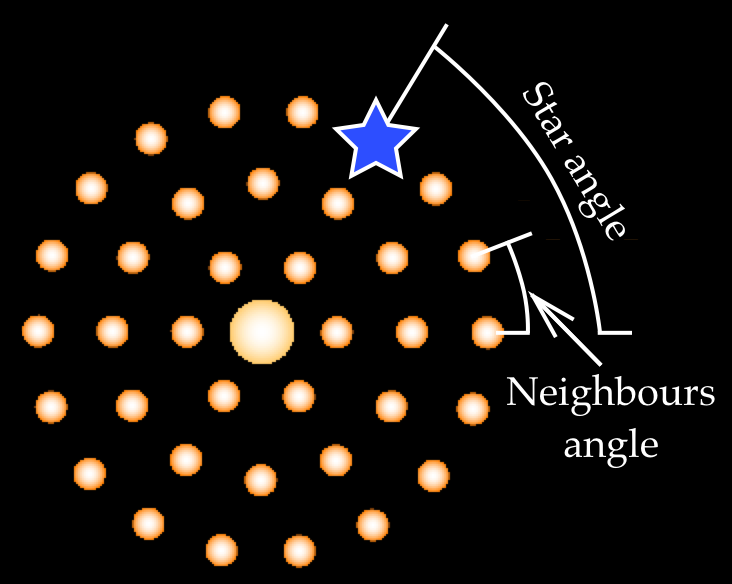
Figure 11: Calculating star angle for the blue star. The star is in the third ring, which has 18 stars. The angle between two neighbours is thus \(360 \degree / 18 = 20 \degree\). Since our blue star is the fourth star along the ring, the starNumber index is 3 and star angle is \(3 \times 20 \degree = 60 \degree\).

Calculating star’s position

It has been a long preparation but now we are ready to calculate the initial position of the star:

// x coordinate
positions[iStar * 3] = distanceFromCenter * Math.cos(starAngle) *
                           Math.cos(galaxyAngleRadians);

// y coordinate
positions[iStar * 3 + 1] = distanceFromCenter * Math.sin(starAngle);

// z coordinate
positions[iStar * 3 + 2] = -distanceFromCenter * Math.cos(starAngle) *
                           Math.sin(galaxyAngleRadians);

In code above we assign x, y and z coordinates to the elements of positions array for the star with index iStar. This index is 0 for the first star, 1 for the second star, 10 for the eleventh star and so on. I admit, the math looks a bit intimidating, but we can understand it with trigonometry and two pictures.

To calculate the star’s position we need three numbers, which we found earlier:

1. distanceFromCenter: Distance of the star from the center of the galaxy (Fig. 9),

2. starAngle: Star angle (Fig. 11),

3. galaxyAngleRadians: Galaxy inclination angle (Fig. 8).

For simplicity, let’s first ignore galaxyAngleRadians, which means the galaxy is not tilted and all the stars lie in the X-Y plane, as shown on Fig 12.

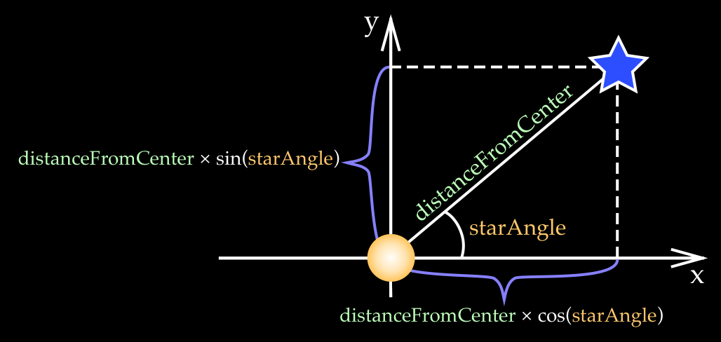
Figure 12: Calculating a star's position when the galaxy is not tilted and all stars are in the X-Y plane.

Then, we multiply the hypotenusedistanceFromCenter by the cosine of the angle to get the x coordinate, and by the sine for the y coordinate. The z coordinate is zero, since the galaxy is not tilted:

// x coordinate
positions[iStar * 3] = distanceFromCenter * Math.cos(starAngle);

// y coordinate
positions[iStar * 3 + 1] = distanceFromCenter * Math.sin(starAngle);

// z coordinate
positions[iStar * 3 + 2] = 0;

Next, we tilt the galaxy around the Y-axis by galaxyAngleRadians angle, as shown on Fig. 13.

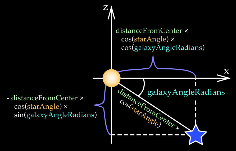
Figure 13: Calculating a star's position of the tilted galaxy.

The key idea here is to think of the galaxy tilt as rotation of the previous x-axis from Fig. 12 around the y-axis. The previous x value distanceFromCenter * cos(starAngle) now becomes the hypotenuse. We then multiply this hypotenuse by cos(galaxyAngleRadians) to get the new x coordinate, and by sin(galaxyAngleRadians) to find the z coordinate. The y-coordinate does not change because the galaxy is tilted around the y-axis:

// x coordinate
positions[iStar * 3] = distanceFromCenter * Math.cos(starAngle) *
                           Math.cos(galaxyAngleRadians);

// y coordinate
positions[iStar * 3 + 1] = distanceFromCenter * Math.sin(starAngle);

// z coordinate
positions[iStar * 3 + 2] = -distanceFromCenter * Math.cos(starAngle) *
                           Math.sin(galaxyAngleRadians);

Notice that we use the negative sign for the z coordinate because we chose to tilt the galaxy clockwise.

To be continued…

I will keep extending this article and cover more code from the simulation.

Thanks 👍

• Daniel Price: my Monash astronomy teacher, who wrote the Fortran code and the laboratory manual this simulation is based on.

• Adelle Goodwin, Melanie Hampel, John Lattanzio and Rosemary Mardling: my Monash teachers, who taught me astronomy and how to simulate movement of masses in space.

• webglfundamentals.org: that’s where I learned how to do 3D drawing in the web browser for this simulation. Relevant sections are “Fundamentals”, “2D translation, rotation, scale, matrix math” and “3D”. My 3D code is based on examples from these chapters.

• Galactic Bridges and Tails: a 1972 paper by Alar and Juri Toomre that analyses similar simulations. I mean, just look at the size and quality of the paper, the attention to detail. Imagine amount of work that went to create all those diagrams by hand. I have not seen anything like that.

• 1941 paper by Erik Holmberg: an even earlier simulation that used physical light bulbs and light sensors instead of computers. I’m super lucky to be able just to press buttons on my laptop.