Programming a three-body problem in JavaScript

Please use a newer browser to see the simulation.

Figure eight Sun, Earth and Jupiter Lagrange point L5 Kepler-16 Chaotic

In this tutorial we will program motion of three bodies in HTML and JavaScript. This work is built upon the two-body simulation code. I want to say huge thanks to Dr Rosemary Mardling, who taught me astrophysics in Monash University. This work is based on Rosmary’s ideas and code. As always, feel free to check the full source code, and use it for any purpose.

Three-body simulations

The little buttons under the slider run the following simulations.

Figure eight

This is a stable three-body system discovered by Cris Moore [5]. The system remains stable even if we change the masses of all bodies a little bit, to 0.99 for example. Just for fun, try increasing the speed of this animation by clicking the clock icon and moving the slider. At certain speeds you will see weird stroboscopic effects. Be careful, this can make you dizzy.

Sun, Earth and Jupiter

This simulation uses true masses, velocities and distances of the Sun, Earth and Jupiter. We can measure one period of the Earth’s orbit in the simulation to be around one second (may depend on computer speed and refresh rate of the monitor). This means that the simulation is working correctly, because it is run at one year per second.

Lagrange point L5

Here the Earth is located near a special point in space called the Sun-Jupiter L5 Lagrange point. Notice that the radius of the Earth’s orbit is smaller than that of Jupiter initially. Planets that are closer to the Sun have shorter orbital periods. Therefore, normally, the Earth would overtake Jupiter. We can check this by decreasing Jupiter’s mass and clicking the Reload button on the bottom right of the simulation screen. However, the combined gravity from Jupiter and the Sun traps the Earth, and it is destined to remain at L5 point behind Jupiter.

Kepler-16

This is a simulation of a binary star system that also has a planet with a mass of 1/3 of Jupiter’s. Both binary stars are smaller than the Sun. The orbital plane of the planet is located edge-on to us. Consequently, when the planet moves in front of the stars, it blocks some of their light. This is precisely how this planet was discovered [6]. The simulation tells us that the system appears to be stable, at least in the short term.

Chaotic

This is an example of how an orderly system can quickly become erratic. When the simulation is running on the computer, small calculation and rounding errors accumulate over time and make the system unpredictable. The simulation is so sensitive to small changes that it may even look different when you run it with the same settings but in different browsers.

The coordinate system

Let’s begin implementing our simulation. We will be using a coordinate system with its origin located at the center of mass of the three bodies, as shown in Fig. 1. We use this origin because, as it turns out, the center of mass of any number of bodies remains motionless or moves with constant velocity.

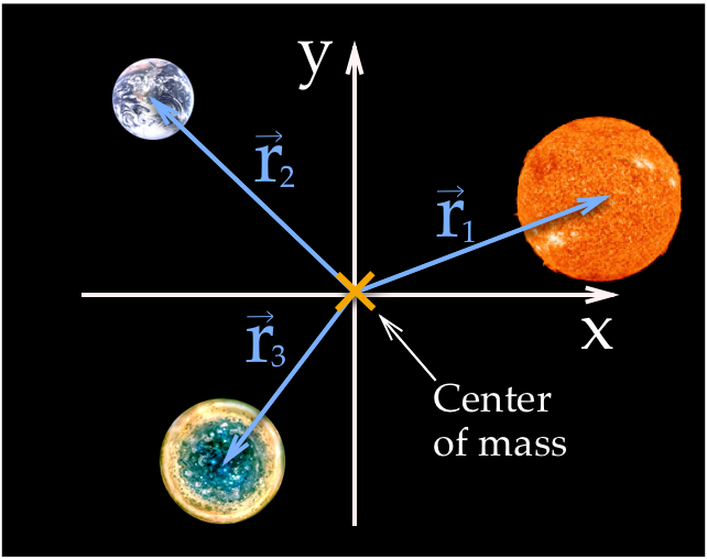
Figure 1: A coordinate system with the origin at the common center of mass of the three bodies.

The equations of motion

The main equation for this simulation is the Newton’s equation of universal gravitation:

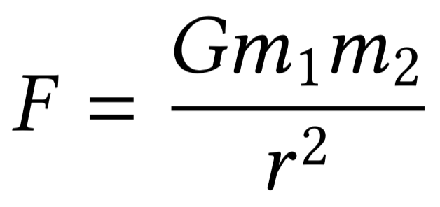(1)

Combining this equation with Newton’s second law F = m a, we can derive three equations of motion:

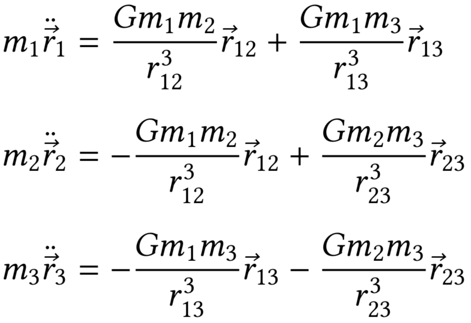(2)

Here the double dots above the variables mean second time derivatives. The vector

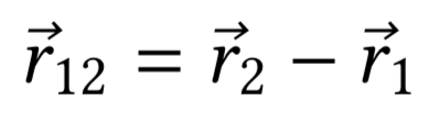(3)

points from the Sun to the Earth. Equation 2 also includes the magnitudes of the vectors, which can be calculated as follows, for the case of the vector r12:

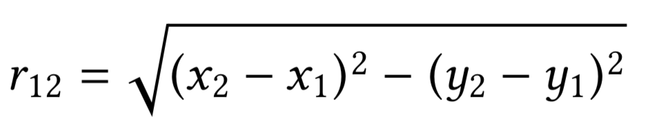(4)

Here x1, y1 and x2, y2 are the coordinates of the Earth and the Sun respectively.

Writing equations of motions in x and y

Equation 2 contains three equations of motion. In order to use the equations in our program we need to write each equation in terms of x and y coordinates. This gives six equations

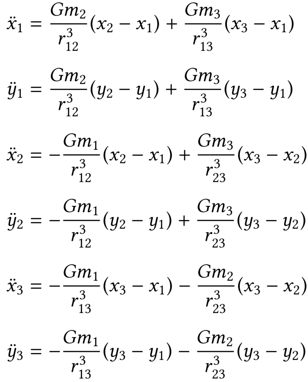(5)

Note the we got rid of the masses on the left-hand sides by dividing both sides by them. The equations look intimidating. However, these are not meant to be used by humans. It is much easier to write these equations in code, since they contain a lot of repetitions. But before we do this, we need to convert the equation into a computer readable form.

Converting the equations to first order

Equation 5 is a system of six second order differential equations. In order to be solved numerically, we need to convert the equations into twelve first order ones. This reduction of order is done by first introducing twelve new variables u:

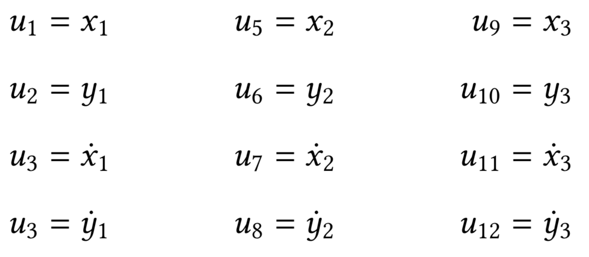(6)

Now we can use the new variables and turn Equation 5 into the following system of first-order differential equations that describe the motion of the three bodies:

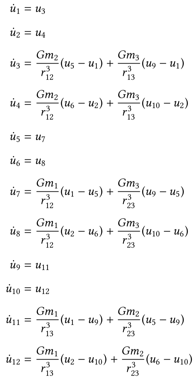(7)

Again, this looks horrific, but in the program this turns into a nice loop that takes care of repetitions.

Programming the equations of motion

We are finally done with algebra and will turn our equations into code. The first thing we need to do is to declare an array that will store that values of those twelve u variables:

// Current state of the system
var state = {
  // State variables used in the differential equations
  // First two elements are x and y positions,
  // and second two are x and y components of velocity
  // repeated for three bodies.
  u: [0, 0, 0, 0, 0, 0, 0, 0, 0, 0, 0, 0]
}

Next, as promised, we turn the long Equation 7 into a much shorter code:

// Calculate the derivatives of the system of ODEs that describe equation of motion of the bodies
function derivative() {
  var du = new Array(initialConditions.bodies * 4);

  // Loop through the bodies
  for (var iBody = 0; iBody < initialConditions.bodies; iBody++) {
    // Starting index for current body in the u array
    var bodyStart = iBody * 4;

    du[bodyStart + 0] = state.u[bodyStart + 0 + 2]; // Velocity x
    du[bodyStart + 1] = state.u[bodyStart + 0 + 3]; // Velocity y
    du[bodyStart + 2] = acceleration(iBody, 0); // Acceleration x
    du[bodyStart + 3] = acceleration(iBody, 1); // Acceleration y
  }

  return du;
}

The function derivative calculates the derivatives of the twelve u variables using Equation 7. For simplicity, the right-hand sides of equation that calculate accelerations, are coded as a separate function:

// Calculates the acceleration of the body 'iFromBody'
// due to gravity from other bodies,
// using Newton's law of gravitation.
//   iFromBody: the index of body. 0 is first body, 1 is second body.
//   coordinate: 0 for x coordinate, 1 for y coordinate
function acceleration(iFromBody, coordinate) {
  var result = 0;
  // Starting index for the body in the u array
  var iFromBodyStart = iFromBody * 4;

  // Loop through the bodies
  for (var iToBody = 0; iToBody < initialConditions.bodies; iToBody++) {
    if (iFromBody === iToBody) { continue; }
    // Starting index for the body in the u array
    var iToBodyStart = iToBody * 4;

    // Distance between the two bodies
    var distanceX = state.u[iToBodyStart + 0] -
      state.u[iFromBodyStart + 0];

    var distanceY = state.u[iToBodyStart + 1] -
      state.u[iFromBodyStart + 1];

    var distance = Math.sqrt(Math.pow(distanceX, 2) +
      Math.pow(distanceY, 2));

    result += constants.gravitationalConstant *
      initialConditions.masses[iToBody] *
      (state.u[iToBodyStart + coordinate] -
        state.u[iFromBodyStart + coordinate]) /
      (Math.pow(distance, 3));
  }

  return result;
}

There are a lot of arrays and indices in this function, and I’ve made a lot of mistakes when I first coded this. But eventually, all bugs were found, removed and carefully released into the wild.

Solving the equations of motion numerically

Next, we need to solve the Equation 7 numerically. In order to do this, we use a popular numerical method called Runge-Kutta. At each frame of our animation, we call the rungeKutta.calculate function and it updates our variables u with new positions and velocities of the three bodies.

// The main function that is called on every animation frame.
// It calculates and updates the current positions of the bodies
function updatePosition(timestep) {
  rungeKutta.calculate(timestep, state.u, derivative);
}

Before the first run, however, we need to choose some initial positions and velocities of the Sun, Earth and Jupiter and store them in the u array.

Drawing the bodies on screen

At each frame of the animation, we calculate new positions of the three bodies in the u array. These position are turned into coordinates of the bodies on computer screen. Here we use the same drawing techniques that we discussed in the harmonic oscillator tutorial.

📚📖✨

If you are into science fiction, The Three-Body Problem novel by Liu Cixin and the other two books of the trilogy could be worth your time.

Credits

1. This work is based on code and lectures by Dr Rosemary Mardling from Monash University.

2. “The Blue Marble” image: NASA/Apollo 17 crew; taken by either Harrison Schmitt or Ron Evans, source, source.

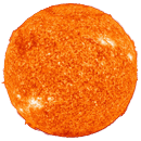
3. “The Sun photographed at 304 angstroms” image: NASA/SDO (AIA), source, source.

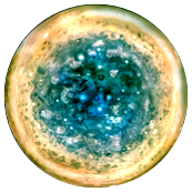
4. “Jupiter’s South Pole” image: NASA/JPL-Caltech/SwRI/MSSS/Betsy Asher Hall/Gervasio Robles, source.

5. Figure eight orbit: Moore, C. 1993, Phys. Rev. Lett., 70, 3675.

6. Kepler-16 system: Doyle, L. R., Carter, J. A., Fabrycky, D. C., et al. 2011, Science, 333, 1602.

References

• The complete source code of the three-body problem simulation.